How to Find Maximum Likelihood Estimators for Mean & Standard Deviation

Now that we know what a likelihood is we turn our focus to Maximum Likelihood Estimator (MLE), which simply maximizes the likelihood function.

We will use the likelihood of a normal distribution to find the optimal values for mean \(\mu\) and standard deviation \(\sigma\) given an observation \(x\), i.e., \(L(\mu, \sigma~|~x)\).

---

MLE for \(\mu\)

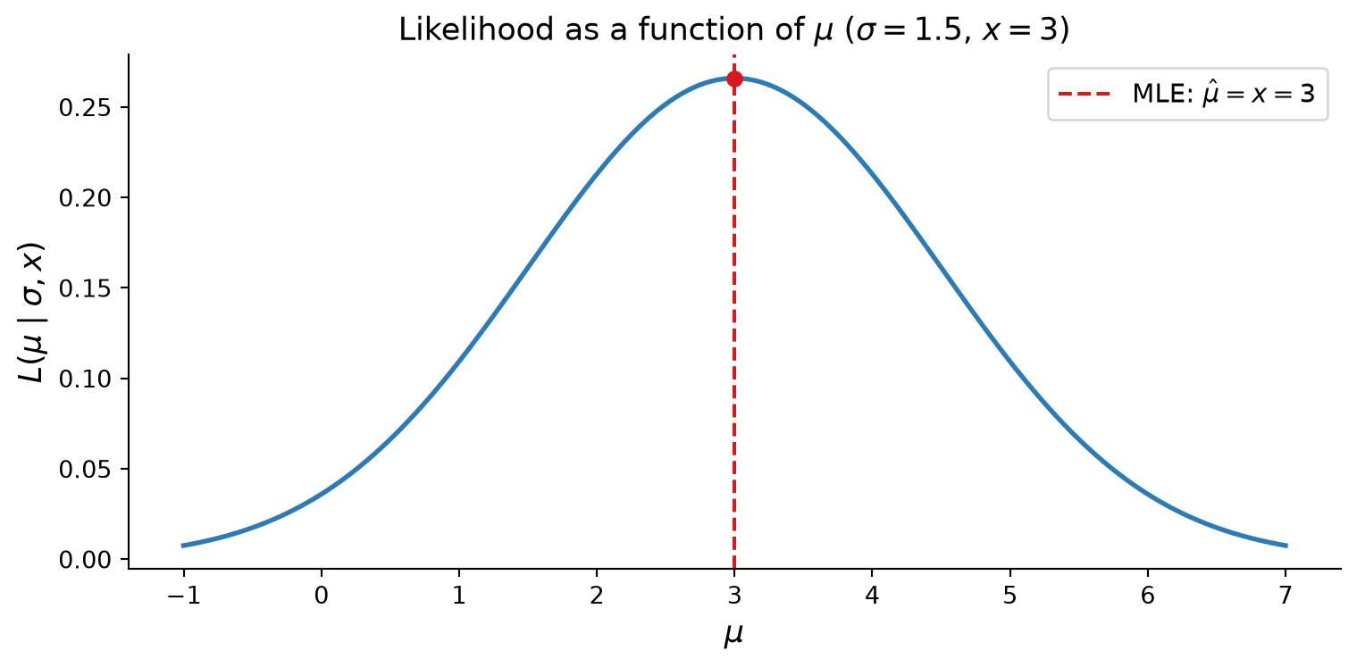
If we fix \(\sigma\) as given and plug in many \(\mu\) values into our normal likelihood function, we get multiple likelihood values:

\[L(\mu\text{'s}~|~\sigma, x)\]

We then check which \(\mu\) gives the maximum likelihood. Note that the peak is when the slope of the curve is 0.

import numpy as np
import matplotlib.pyplot as plt
from scipy.stats import norm

# Observed data point and fixed sigma
x_obs = 3.0
sigma_fixed = 1.5

# Range of mu values to try
mu_vals = np.linspace(-1, 7, 500)
likelihoods = norm.pdf(x_obs, loc=mu_vals, scale=sigma_fixed)

mu_mle = x_obs  # MLE for mu equals the observation

fig, ax = plt.subplots(figsize=(8, 4))
ax.plot(mu_vals, likelihoods, color="#2c7bb6", linewidth=2)
ax.axvline(mu_mle, color="#d7191c", linestyle="--", linewidth=1.5,
           label=r"MLE: $\hat{\mu} = x = 3$")
ax.scatter([mu_mle], [norm.pdf(x_obs, loc=mu_mle, scale=sigma_fixed)],
           color="#d7191c", zorder=5)

ax.set_xlabel(r"$\mu$", fontsize=13)
ax.set_ylabel(r"$L(\mu \mid \sigma, x)$", fontsize=13)
ax.set_title(r"Likelihood as a function of $\mu$ ($\sigma = 1.5$, $x = 3$)", fontsize=13)
ax.legend(fontsize=11)
ax.spines[["top", "right"]].set_visible(False)
plt.tight_layout()
plt.show()

Figure 1: Likelihood as a function of μ (σ fixed, x = 3). The peak marks the MLE.

---

MLE for \(\sigma\)

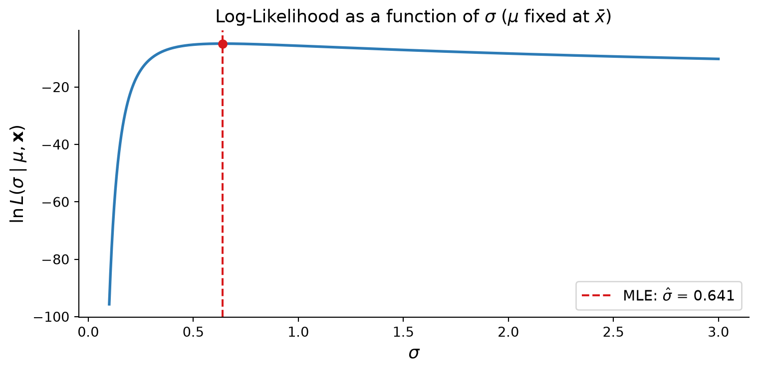
We do the same for \(\sigma\), this time by fixing \(\mu\):

\[L(\sigma\text{'s}~|~\mu, x)\]

sigma_vals = np.linspace(0.2, 6, 500)
likelihoods_sigma = norm.pdf(x_obs, loc=mu_mle, scale=sigma_vals)

# For a single observation the likelihood keeps rising as sigma -> inf,
# so we show a multi-observation case to get a proper peak.
np.random.seed(42)
data = np.array([2.1, 3.4, 2.8, 3.9, 2.5])
n = len(data)

def log_likelihood(mu, sigma, data):
    return np.sum(norm.logpdf(data, loc=mu, scale=sigma))

mu_hat = np.mean(data)
sigma_hat = np.std(data, ddof=0)  # MLE uses n in denominator

sigma_range = np.linspace(0.1, 3, 500)
ll_vals = [log_likelihood(mu_hat, s, data) for s in sigma_range]

fig, ax = plt.subplots(figsize=(8, 4))
ax.plot(sigma_range, ll_vals, color="#2c7bb6", linewidth=2)
ax.axvline(sigma_hat, color="#d7191c", linestyle="--", linewidth=1.5,
           label=rf"MLE: $\hat{{\sigma}}$ = {sigma_hat:.3f}")
ax.scatter([sigma_hat], [log_likelihood(mu_hat, sigma_hat, data)],
           color="#d7191c", zorder=5)

ax.set_xlabel(r"$\sigma$", fontsize=13)
ax.set_ylabel(r"$\ln L(\sigma \mid \mu, \mathbf{x})$", fontsize=13)
ax.set_title(r"Log-Likelihood as a function of $\sigma$ ($\mu$ fixed at $\bar{x}$)", fontsize=13)
ax.legend(fontsize=11)
ax.spines[["top", "right"]].set_visible(False)
plt.tight_layout()
plt.show()

Figure 2: Likelihood as a function of σ (μ fixed at x = 3). The peak marks the MLE.

---

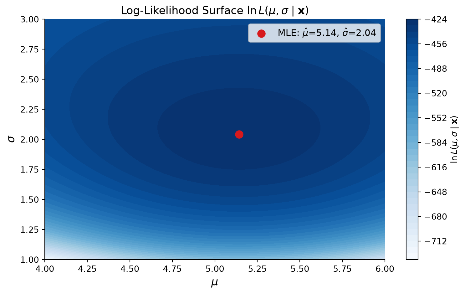
Expanding to \(n\) Observations

Because each sample is independent, the likelihood for \(n\) samples is:

\[ \begin{aligned} L(\mu, \sigma~|~x_1, x_2, \ldots, x_n) &= L(\mu, \sigma~|~x_1) \cdots L(\mu, \sigma~|~x_n) \\ &= \frac{1}{\sqrt{2\pi\sigma^2}}e^{-\frac{(x_1-\mu)^2}{2\sigma^2}} \cdots \frac{1}{\sqrt{2\pi\sigma^2}}e^{-\frac{(x_n-\mu)^2}{2\sigma^2}} \end{aligned} \]

---

Log-Likelihood

One trick is to take the derivative of \(\ln L\) instead of \(L\) — the peaks are identical but the math is far simpler.

\[ \begin{aligned} \ln[L(\mu, \sigma~|~x_1, \ldots, x_n)] &= \ln[L(\mu,\sigma~|~x_1)] + \cdots + \ln[L(\mu,\sigma~|~x_n)] \\ &= \left(-\tfrac{1}{2}\ln(2\pi\sigma^2) - \frac{(x_1-\mu)^2}{2\sigma^2}\right) + \cdots + \left(-\tfrac{1}{2}\ln(2\pi\sigma^2) - \frac{(x_n-\mu)^2}{2\sigma^2}\right) \\ &= -\frac{n}{2}\ln(2\pi) - n\ln\sigma - \frac{1}{2\sigma^2}\sum_{i=1}^{n}(x_i - \mu)^2 \end{aligned} \]

---

Solving for \(\hat{\mu}\)

Take the partial derivative with respect to \(\mu\) and set to zero:

\[ \begin{aligned} \frac{\partial}{\partial \mu}\ln L &= \frac{1}{\sigma^2}\!\left(\sum_{i=1}^{n}x_i - n\mu\right) = 0 \\ &\Rightarrow\quad \boxed{\hat{\mu} = \frac{1}{n}\sum_{i=1}^{n}x_i} \end{aligned} \]

The MLE for \(\mu\) is simply the sample mean.

---

Solving for \(\hat{\sigma}\)

Take the partial derivative with respect to \(\sigma\) and set to zero:

\[ \begin{aligned} \frac{\partial}{\partial \sigma}\ln L &= -\frac{n}{\sigma} + \frac{1}{\sigma^3}\sum_{i=1}^{n}(x_i-\mu)^2 = 0 \\ &\Rightarrow\quad \boxed{\hat{\sigma} = \sqrt{\frac{1}{n}\sum_{i=1}^{n}(x_i-\mu)^2}} \end{aligned} \]

The MLE for \(\sigma\) is the population standard deviation of the data.

---

Verification with Python

import numpy as np
from scipy.optimize import minimize_scalar, minimize

np.random.seed(0)
data = np.random.normal(loc=5, scale=2, size=200)

# Analytical MLEs
mu_hat_analytic    = np.mean(data)
sigma_hat_analytic = np.std(data, ddof=0)   # MLE uses 1/n

# Numerical MLE via scipy (minimize negative log-likelihood)
def neg_log_lik(params, data):
    mu, log_sigma = params
    sigma = np.exp(log_sigma)               # ensure sigma > 0
    return -np.sum(norm.logpdf(data, loc=mu, scale=sigma))

result = minimize(neg_log_lik, x0=[0, 0], args=(data,), method="Nelder-Mead")
mu_hat_num    = result.x[0]
sigma_hat_num = np.exp(result.x[1])

print(f"Analytical MLE  →  μ̂ = {mu_hat_analytic:.4f},  σ̂ = {sigma_hat_analytic:.4f}")
print(f"Numerical  MLE  →  μ̂ = {mu_hat_num:.4f},  σ̂ = {sigma_hat_num:.4f}")
print(f"True values     →  μ  = 5.0000,  σ  = 2.0000")

Analytical MLE  →  μ̂ = 5.1418,  σ̂ = 2.0428
Numerical  MLE  →  μ̂ = 5.1418,  σ̂ = 2.0428
True values     →  μ  = 5.0000,  σ  = 2.0000

---

Log-Likelihood Surface

The plot below shows the log-likelihood surface over a grid of \((\mu, \sigma)\) values. The red dot marks the MLE — the peak of the surface.

mu_grid    = np.linspace(4, 6, 200)
sigma_grid = np.linspace(1, 3, 200)
MU, SIG    = np.meshgrid(mu_grid, sigma_grid)

LL = np.array([
    [np.sum(norm.logpdf(data, loc=m, scale=s)) for m in mu_grid]
    for s in sigma_grid
])

fig, ax = plt.subplots(figsize=(8, 5))
cp = ax.contourf(MU, SIG, LL, levels=40, cmap="Blues")
fig.colorbar(cp, ax=ax, label=r"$\ln L(\mu, \sigma \mid \mathbf{x})$")
ax.scatter([mu_hat_analytic], [sigma_hat_analytic],
           color="#d7191c", s=80, zorder=5,
           label=rf"MLE: $\hat{{\mu}}$={mu_hat_analytic:.2f}, $\hat{{\sigma}}$={sigma_hat_analytic:.2f}")
ax.set_xlabel(r"$\mu$", fontsize=13)
ax.set_ylabel(r"$\sigma$", fontsize=13)
ax.set_title(r"Log-Likelihood Surface $\ln L(\mu, \sigma \mid \mathbf{x})$", fontsize=13)
ax.legend(fontsize=11)
ax.spines[["top", "right"]].set_visible(False)
plt.tight_layout()
plt.show()

Figure 3: Log-likelihood surface for μ and σ. The MLE sits at the peak.