Classification Trees

Now we know what Classification Trees are let’s see how to train and make predictions. We will use the wine dataset from sklearn

import pandas as pd
from sklearn.datasets import load_wine
import seaborn as sns
import matplotlib.pyplot as plt
from sklearn.model_selection import train_test_split
from sklearn.tree import DecisionTreeClassifier
from sklearn.metrics import accuracy_score
from sklearn.metrics import confusion_matrix
from sklearn import tree
from sklearn.metrics import accuracy_score, precision_score, recall_score, f1_score
from sklearn.metrics import classification_report

# Load wine data in numpy array
X, y = load_wine(return_X_y = True)
X.shape # 178 instances

(178, 13)

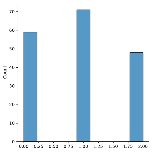
# Check distribution our target
sns.displot(y)

# Split into training set and test set
X_train, X_test, y_train, y_test = train_test_split(X, y, test_size = .20, random_state=0)
X_train.shape # 142 instances

(142, 13)

# Define our model
dt_classifier = DecisionTreeClassifier(max_depth = 2) 

# Train
dt_classifier.fit(X_train, y_train)

DecisionTreeClassifier(max_depth=2)

In a Jupyter environment, please rerun this cell to show the HTML representation or trust the notebook.
On GitHub, the HTML representation is unable to render, please try loading this page with nbviewer.org.

DecisionTreeClassifier

?Documentation for DecisionTreeClassifieriFitted

Parameters

	max_depth max_depth: int, default=None The maximum depth of the tree. If None, then nodes are expanded until all leaves are pure or until all leaves contain less than min_samples_split samples.	2
	criterion criterion: {"gini", "entropy", "log_loss"}, default="gini" The function to measure the quality of a split. Supported criteria are "gini" for the Gini impurity and "log_loss" and "entropy" both for the Shannon information gain, see :ref:`tree_mathematical_formulation`.	'gini'
	splitter splitter: {"best", "random"}, default="best" The strategy used to choose the split at each node. Supported strategies are "best" to choose the best split and "random" to choose the best random split.	'best'
	min_samples_split min_samples_split: int or float, default=2 The minimum number of samples required to split an internal node: - If int, then consider `min_samples_split` as the minimum number. - If float, then `min_samples_split` is a fraction and `ceil(min_samples_split * n_samples)` are the minimum number of samples for each split. .. versionchanged:: 0.18 Added float values for fractions.	2
	min_samples_leaf min_samples_leaf: int or float, default=1 The minimum number of samples required to be at a leaf node. A split point at any depth will only be considered if it leaves at least ``min_samples_leaf`` training samples in each of the left and right branches. This may have the effect of smoothing the model, especially in regression. - If int, then consider `min_samples_leaf` as the minimum number. - If float, then `min_samples_leaf` is a fraction and `ceil(min_samples_leaf * n_samples)` are the minimum number of samples for each node. .. versionchanged:: 0.18 Added float values for fractions.	1
	min_weight_fraction_leaf min_weight_fraction_leaf: float, default=0.0 The minimum weighted fraction of the sum total of weights (of all the input samples) required to be at a leaf node. Samples have equal weight when sample_weight is not provided.	0.0
	max_features max_features: int, float or {"sqrt", "log2"}, default=None The number of features to consider when looking for the best split: - If int, then consider `max_features` features at each split. - If float, then `max_features` is a fraction and `max(1, int(max_features * n_features_in_))` features are considered at each split. - If "sqrt", then `max_features=sqrt(n_features)`. - If "log2", then `max_features=log2(n_features)`. - If None, then `max_features=n_features`. .. note:: The search for a split does not stop until at least one valid partition of the node samples is found, even if it requires to effectively inspect more than ``max_features`` features.	None
	random_state random_state: int, RandomState instance or None, default=None Controls the randomness of the estimator. The features are always randomly permuted at each split, even if ``splitter`` is set to ``"best"``. When ``max_features < n_features``, the algorithm will select ``max_features`` at random at each split before finding the best split among them. But the best found split may vary across different runs, even if ``max_features=n_features``. That is the case, if the improvement of the criterion is identical for several splits and one split has to be selected at random. To obtain a deterministic behaviour during fitting, ``random_state`` has to be fixed to an integer. See :term:`Glossary <random_state>` for details.	None
	max_leaf_nodes max_leaf_nodes: int, default=None Grow a tree with ``max_leaf_nodes`` in best-first fashion. Best nodes are defined as relative reduction in impurity. If None then unlimited number of leaf nodes.	None
	min_impurity_decrease min_impurity_decrease: float, default=0.0 A node will be split if this split induces a decrease of the impurity greater than or equal to this value. The weighted impurity decrease equation is the following:: N_t / N * (impurity - N_t_R / N_t * right_impurity - N_t_L / N_t * left_impurity) where ``N`` is the total number of samples, ``N_t`` is the number of samples at the current node, ``N_t_L`` is the number of samples in the left child, and ``N_t_R`` is the number of samples in the right child. ``N``, ``N_t``, ``N_t_R`` and ``N_t_L`` all refer to the weighted sum, if ``sample_weight`` is passed. .. versionadded:: 0.19	0.0
	class_weight class_weight: dict, list of dict or "balanced", default=None Weights associated with classes in the form ``{class_label: weight}``. If None, all classes are supposed to have weight one. For multi-output problems, a list of dicts can be provided in the same order as the columns of y. Note that for multioutput (including multilabel) weights should be defined for each class of every column in its own dict. For example, for four-class multilabel classification weights should be [{0: 1, 1: 1}, {0: 1, 1: 5}, {0: 1, 1: 1}, {0: 1, 1: 1}] instead of [{1:1}, {2:5}, {3:1}, {4:1}]. The "balanced" mode uses the values of y to automatically adjust weights inversely proportional to class frequencies in the input data as ``n_samples / (n_classes * np.bincount(y))`` For multi-output, the weights of each column of y will be multiplied. Note that these weights will be multiplied with sample_weight (passed through the fit method) if sample_weight is specified.	None
	ccp_alpha ccp_alpha: non-negative float, default=0.0 Complexity parameter used for Minimal Cost-Complexity Pruning. The subtree with the largest cost complexity that is smaller than ``ccp_alpha`` will be chosen. By default, no pruning is performed. See :ref:`minimal_cost_complexity_pruning` for details. See :ref:`sphx_glr_auto_examples_tree_plot_cost_complexity_pruning.py` for an example of such pruning. .. versionadded:: 0.22	0.0
	monotonic_cst monotonic_cst: array-like of int of shape (n_features), default=None Indicates the monotonicity constraint to enforce on each feature. - 1: monotonic increase - 0: no constraint - -1: monotonic decrease If monotonic_cst is None, no constraints are applied. Monotonicity constraints are not supported for: - multiclass classifications (i.e. when `n_classes > 2`), - multioutput classifications (i.e. when `n_outputs_ > 1`). The constraints hold over the probability of the positive class. Read more in the :ref:`User Guide <monotonic_cst_gbdt>`. .. versionadded:: 1.4	None

Fitted attributes

Name	Type	Value
classes_ classes_: ndarray of shape (n_classes,) or list of ndarray The classes labels (single output problem), or a list of arrays of class labels (multi-output problem).	ndarray[int64](3,)	[0,1,2]
feature_importances_ feature_importances_: ndarray of shape (n_features,) The impurity-based feature importances. The higher, the more important the feature. The importance of a feature is computed as the (normalized) total reduction of the criterion brought by that feature. It is also known as the Gini importance [4]_. Warning: impurity-based feature importances can be misleading for high cardinality features (many unique values). See :func:`sklearn.inspection.permutation_importance` as an alternative.	ndarray[float64](13,)	[0.,0.,0.,...,0.,0.,0.]
max_features_ max_features_: int The inferred value of max_features.	int	13
n_classes_ n_classes_: int or list of int The number of classes (for single output problems), or a list containing the number of classes for each output (for multi-output problems).	int64	np.int64(3)
n_features_in_ n_features_in_: int Number of features seen during :term:`fit`. .. versionadded:: 0.24	int	13
n_outputs_ n_outputs_: int The number of outputs when ``fit`` is performed.	int	1
tree_ tree_: Tree instance The underlying Tree object. Please refer to ``help(sklearn.tree._tree.Tree)`` for attributes of Tree object and :ref:`sphx_glr_auto_examples_tree_plot_unveil_tree_structure.py` for basic usage of these attributes.	Tree	<sklearn.tree...t 0x11c2779f0>

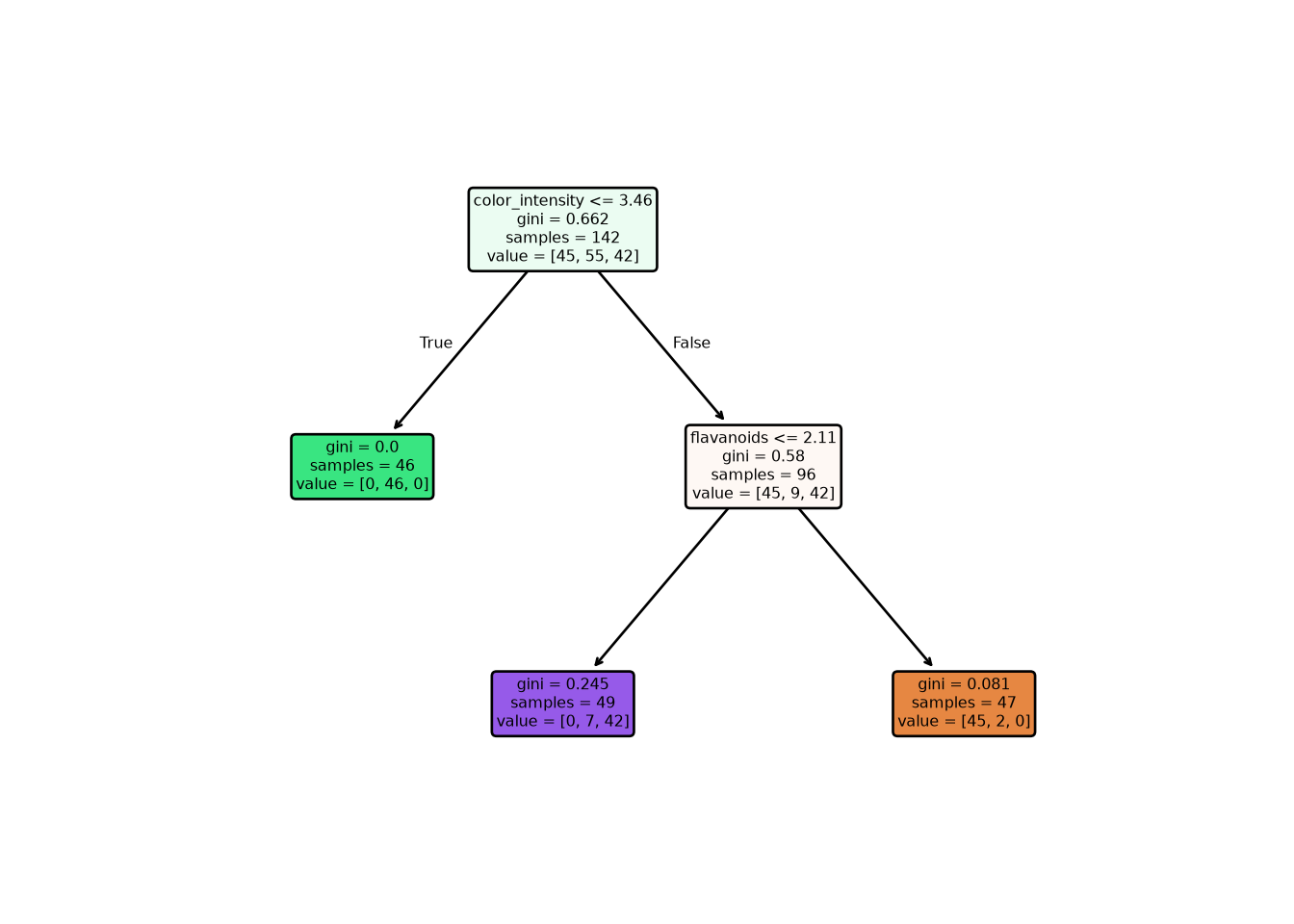
Note the max_depth hyperparameter from DecisionTreeClassifier was set to 2. We used 2 arbitrarily but we could have used cross validation to select the best depth.

With our trained model we can use predict to predict the classes:

# Predict
y_train_predict = dt_classifier.predict(X_train)

Let’s visualize our tree:

wine = load_wine()

plt.figure()
tree.plot_tree(
  dt_classifier,
  feature_names = wine.feature_names,
  filled = True, 
  fontsize=6, 
  rounded = True
  )
plt.show()

color_intensity <= 3.82: threshold that separates into different nodes
gini: Gini Impurity
samples: number of observations for each node
value: number of classifications that fall into each group

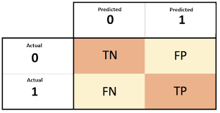
We trained our Classification Tree and got our predictions. The last step is to evaluate our model but how? We use a Confusion Matrix:

Let’s assume we have two classes and let 0 be the negative class and 1 the positive class. Each row is an actual class and each column is the predicted class. Depending on how the classifications were made we divide them into four different categories:

\(TN = \frac{correctly~classified~as~negative}{negative~class}\)
\(FP = \frac{incorrectly~classified~as~positive}{negative~class}\)
\(FN = \frac{incorrectly~classified~as~negative}{positive~class}\)
\(TP = \frac{correctly~classified~as~positive}{positive~class}\)

Next, we discuss three different ways from a confusion matrix to see how good your classification tree is:

\(Accuracy = \frac{TN+TP}{TN+FP+FN+TP}\)
\(Precision = \frac{TP}{FP+TP}\)
\(Recall = \frac{TP}{FN+TP}\)

Based on the confusion matrix it seems natural to use Accuracy but consider the case where we have 9 negative and 1 positive observations and let’s say there is a silly model that always classifies as negative. Then the accuracy is 90% (TN: 9, FP: 0, FN: 1, TP: 0 => \(\frac{9+1}{9+0+1+0}\)). Hence accuracy is not always a good metric especially when the classes are imbalanced. This is why we need a better metric like Precision. As you can see from the formula, the denominator takes all predicted cases both false positive and true positive. Out of these we want to find only the true positives, hence Precision is the accuracy of the positive predictions.

However Precision is also not perfect. If we only have one positive prediction and if that is true positive, then we have 100% Precision (\(\frac{1}{1+0}\)). This is why we report Recall aka Sensitivity or True Positive Rate along with Precision. Recall only differs by the denominator: the number of true positives out of all the actual positive instances.

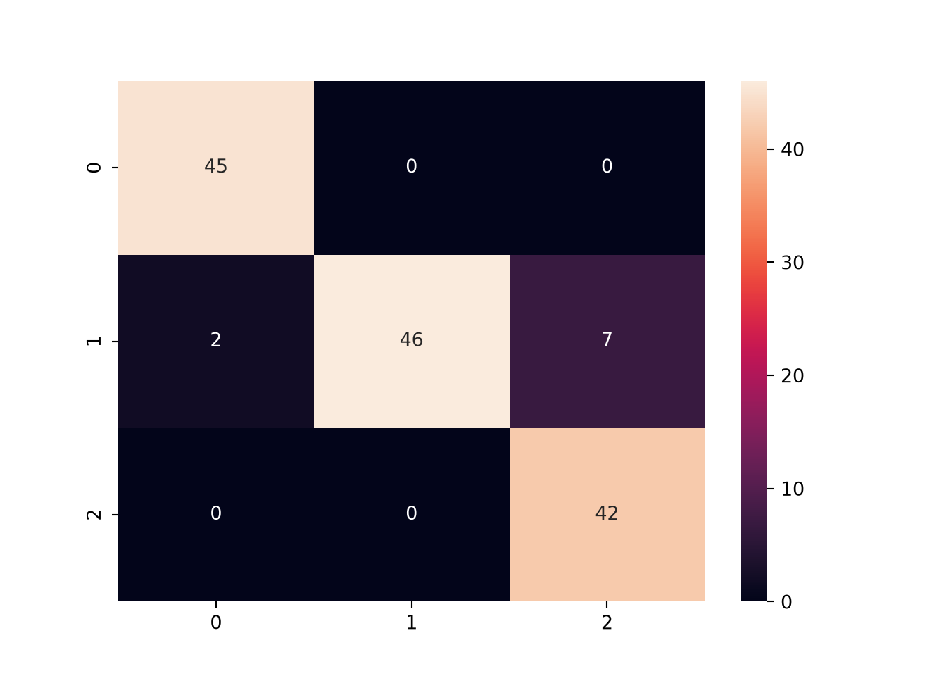
This is the confusion matrix for our wine data:

confusion_matrix(y_train, y_train_predict)

array([[45,  0,  0],
       [ 2, 46,  7],
       [ 0,  0, 42]])

Note that this matrix is 3 by 3 as we have three classes instead of two. We call this a multi-class classification. We apply the same logic as we did for 2 by 2 but we just need to break each of the three classes into positive or negative, respectively. If we assume class0 is positive, then

TP = classified as class0 when the actual is class0 = 45
FP = classified as class0 when the actual is not = 2 + 0 = 2
TN = classified as not class0 (class1 or class2) when the actual is not = 46 + 7 + 0 + 42 = 95
FN = classified as not class0 when the actual is class0 = 0 + 0 = 0
Precision = \(\frac{45}{45+2}=0.96\)
Recall = \(\frac{45}{45+0}=1.00\)

## Evaluation
# Accuracy
accuracy_score(y_train, y_train_predict)

0.9366197183098591

sns.heatmap(confusion_matrix(y_train, y_train_predict), annot = True)
plt.show()

print(classification_report(y_train, y_train_predict, target_names=['Class 0', 'Class 1', 'Class 2']))

              precision    recall  f1-score   support

     Class 0       0.96      1.00      0.98        45
     Class 1       1.00      0.84      0.91        55
     Class 2       0.86      1.00      0.92        42

    accuracy                           0.94       142
   macro avg       0.94      0.95      0.94       142
weighted avg       0.94      0.94      0.94       142

macro avg is calculated as the unweighted mean of f1-scores from each class : \(\frac{0.98+0.91+0.92}{3}=0.94\)

weighted avg is calculated as the weighted mean of the number of samples for each class

Now that we we know Precision and Recall, let’s dive in a little bit deeper. Because there is a trade-off between Precision and Recall, generally we can’t have both perfect metrics. However there are cases where we care mostly just about Precision or Recall and it is OK to have the other showing a low value.

For instance, let’s say there is a COVID-19 testing kit that tells a potential patient whether or not they have COVID. In this context, a false positive means even though the patient is COVID negative, the kit says positive. On the other hand, a false negative means even though the patient is COVID positive, the kit says negative. Between false positive and false negative which one do you think is more critical? It would be false negative as that patient carries the real COVID but will feel comfortable to hang out simply because the kit says the opposite/healthy which will result in spreading COVID. On the flip side, it is relatively OK to have higher false positive because the patient will be cautious and being cautious will not harm anyone. Hence, we need to have a high recall but it is OK to have low precision.

Another example would be to test a an AI model tells if a person is guilty or not. Assuming positive is guilty and negative not guilty, false positive means even though the person is innocent, the classifier says guilty. False negative means even though the person is guilty, the classifier says innocent. Of these two, let’s assume that the stakeholders considered false positive being the worst case because no innocent people should be classified as guilty. Hence, we need to have high precision but it is relatively OK to have low recall.